DMM Varkon^® Tutorial
A Beginner's Guide to the Varkon Parametric Modeling and CAD Application Development System
By David M. MacMillan

17. Example: Pendulum Demo

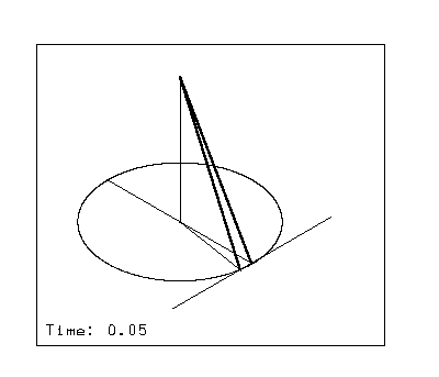
NOTE: This physics of this animation are WRONG. This demo is intended to show the motion of two superimposed pendulums (conical, planar) as described below. What it shows instead is the motion of a conical pendulum (correctly) and the motion of a planar pendulum as if that pendulum exhibited true simple harmonic motion. Although simple harmonic motion is a good approximation for pendulum motion, real planar pendulums move very slightly differently. I'm currently working on a correction for this. However, since the point of this page is to show Varkon code rather than physics, for now I'm including this demo. I would ask only that you don't take this demo as an accurate model of pendulum motion.

This animated GIF shows the relationship between the motions of two different types of pendulums of equal length (just under a meter) and period (two seconds for a full period). One of the pendulums is a conventional or "planar" pendulum swinging back and forth in a vertical plane. The other pendulum is a so-called "conical" pendulum whose motion describes a cone. The motion of the conical pendulum is uniform circular motion. The motion of the planar pendulum approximates (but is not entirely equivalent to) "harmonic" or sinusoidal motion. The animation demonstrates graphically that the nearly harmonic motion is a projection of uniform circular motion.

In order to more clearly show these motions, the amplitude of these pendulums in this animation is 30 degrees (measured as a half-swing). Such an amplitude is much greater than that common in real clocks, where amplitudes for a seconds-beating pendulum might rarely exceed three degrees.

One full cycle of this animation consists of a complete swing of the conical pendulum or a full (right-left-right) period of the planar pendulum and runs from Time: 0.00 to Time: 2.00. The animation should loop through this cycle four times. If the animation appears to get stuck, try moving the mouse pointer into the window and pressing the ENTER key. To run the animation again, click on your browser's RELOAD button.

Aside: The animation actually begins on image 1 at 0:05, not on image 0. If it began on image 0, then in each loop the final image at 2:00 would visually be repeated by a graphically identical image at 0:00, causing an extra visual "beat" in the animation. This means that the image computed for time 0, the opening position, is not actually present in this animated GIF.

Implementation

Active Module

The active module is just a stub which calls the animation driver, pmdemo1():

GLOBAL DRAWING MODULE pmshow();


BEGINMODULE

  part(#1,pmdemo1());

ENDMODULE

Animation Driver

This is the animation driver, pmdemo1.MBS.

! pmdemo1.MBS

! This driver for penddemo.MBS displays a 2D drawing with a border
! in which a single isometric view of the pendulum demo is animated.

! This border is necessary to ensure that the plot files generated from
! this animation all have the same frame of reference.

! This module is placed in the public domain by its author,
! David M. MacMillan

global drawing module pmdemo1 (
);

! pendulum parameters
! Note: offsets are not done as vec(x,y,z) because Varkon disallows
!       3-value vectors in a 2-D drawing module such as this one.
float xoff;  ! X,Y,Z offsets of pendulum 
float yoff;  ! Offsets are of the point at the center of the circle
float zoff;  ! described by the tip of the conical pendulum
float hp;    ! half period, or one swing of pendulum 1, in seconds
float amp;   ! pendulum amplitude (max half swing), in degrees

! overall size of the model as calculated by the model
float xsize; 
float ysize;
float zsize;

! simulation parameters
float t;      ! elapsed time from 0, in seconds
float maxt;   ! total time to be simulated, in seconds
float inct;   ! time-resolution, in seconds

! display strings
string timestring*32;

! plot file 
string plotfile*132;
int    plotnum;

constant float fudge = 0.0001;

! lower left and upper right corners of the drawing border
float  xmin;
float  xmax;
float  ymin;
float  ymax;

! the space between views (2D window on screen)
constant float viewspace = 200;

! drawing size as vectors, for use in plotting
vector minpos;
vector maxpos;

! miscellaneous constants
constant float norot    = 0;    ! do not rotate
constant float isoangle = 35.266666; ! angle between the edge of an
                                     ! isometrically projected cube and
                                     ! the plane of projection (35 deg 16 min)


beginmodule

! Clear Varkon's cache, to be sure to always load the latest
! compiled version of each module.
clear_pm ();

! Set curve plotting accuracy.  -0.1 < cacc < 100; default 1.0
cacc_view(100);

! Choose the pendulum's period.
hp   := 1;

! Let's just put the demo at the origin.
xoff := 0;
yoff := 0;
zoff := 0;

amp   := 30;    ! <= 3 for realistic modern clocks; 
                ! 30 or more for exaggerated demo
maxt  := 16;
inct  := 0.05;

t       := 0;
plotnum := 0;

! while (t <= maxt) 
! (given that maxt is known, perhaps a FOR loop would be more appropriate...)
startcycle:

   ! clear the model, so we draw afresh
   clear_gm ();

   ! Set up a local coordinate system in the XY plane which locates
   ! the model (actually, this is just the origin here).
   csys_1p (#1, "iso", vec (xoff, yoff), norot, norot, norot: blank=1);

   ! Invoke the model, rotating it so that it presents an isometric projection
   part (#2, penddemo (hp,                    ! half period
                       amp,                   ! amplitude
                       t,                     ! elapsed time
                       isoangle, -45, 0,      ! isometric view
                       xsize, ysize, zsize),  ! size (to be computed)
             #1);  

   ! Although the border points below could be calculated,
   ! for now they're just derived semi-empirically.
   xmin  := - (xsize / 2) - viewspace; 
   ymin  := -(viewspace * 3);
   xmax  := xsize;
   ymax  := ysize;
   ! Draw a border around the drawing.
   lin_free (#10, vec (xmin, ymin), vec (xmax, ymin));
   lin_free (#11, vec (xmax, ymin), vec (xmax, ymax));
   lin_free (#12, vec (xmax, ymax), vec (xmin, ymax));
   lin_free (#13, vec (xmin, ymax), vec (xmin, ymin));

   ! Write a text string which displays the elapsed simulation time digitally.
   timestring := "Time: " + str (t, 1, 2);
   text (#14, vec (xmin + 50, ymin + 50), 0, timestring: tsize=50, tslant=0);

   ! Plot the current view to a file.
   ! Files are named 0.PLT, 1.PLT, ... n.PLT
   minpos := vec(xmin, ymin);
   maxpos := vec(xmax, ymax);
   plotfile := str(plotnum, 1, 0);
   plotfile := plotfile+".PLT";
   plot_win(minpos, maxpos, plotfile);
   plotnum  := plotnum + 1;

   ! Note: When handling the output, remember that the image is plotted
   ! at full scale - the pendulum is 1 physical meter long.

   ! I'm not entirely sure why the "fudge factor" is necessary, but without
   ! it the loop will not stop exactly at, for example, the half and
   ! full revolution positions (but instead will go one step beyond).
   if t < (maxt - fudge) then
      t := t + inct;
      goto startcycle;
   else
      goto endcycle;
   endif;

endcycle:;

endmodule

Model

This is the model itself, penddemo.MBS.

! penddemo.MBS

! Demonstrate pendulum motion graphically by superimposing
! a conical and a "planar" pendulum.

! Note: We specify period and calculate pendulum length from it because
!       1) period is more important and
!       2) rounding errors in calculating the period from the length
!          result in small but visible discrepancies in the position of
!          pendulums with assumed integral periods.  Similar errors in
!          length will not be perceptible.

! This module is placed in the public domain by its author,
! David M. MacMillan


local geometry module penddemo (
float hp;        ! half-period (one swing), in seconds
float amp;       ! half-swing in degrees
float t;         ! elapsed time t in seconds from 0
float xrot;      ! rotation of model to establish it's local coordinate system
float yrot;
float zrot;
var float xsize; ! computed dimensions of model, to pass back to the caller
var float ysize;
var float zsize
);


! the center of the circle described by the motion of the tip, or
! "center of oscillation," of the conical pendulum
vector cbasectr;    ! vec (xoff, yoff, zoff)

! the pendulum
float  length;      ! effective pendulum length, in mm
float  h;           ! height of suspension point above cbasectr, in mm
float  swingradius; ! radius of circile described by the conical pendulum, in mm
float  cpa;         ! conical pendulum's phase angle
vector pintersect;  ! intersection of swing of planar pendulum with
                    ! plane described by conical pendulum's tip

! gravitational acceleration in mm/sec/sec
constant float g = 9810;   

beginmodule

! Combine the positional offsets into a vector.
! (In this version of this module there are no positional offsets.)
cbasectr := vec (0, 0, 0);

! Create a local coordinate system for this model.
! The rotations used here will have been specified as parameters
! such that the model, as rotated, will present the desired view
! to the XY plane of the module which called us.
csys_1p (#1, "local", cbasectr, xrot, yrot, zrot: blank=1);
mode_local (#1);

! Determine the length of the pendulum
! From Rawlings, _The Science of Clocks and Watches_. 3rd edition, p. 28 
! (or any good text)
!       hp = pi * sqrt (l/g)
! where hp is the half period (one swing) of the pendulum
!        l is the length of the pendulum
!        g is the gravitational constant
! Solving for l, and using the "**" symbol to indicate exponentiation,
! this gives:

length := (g * (hp**2)) / (PI**2);

! Determine the radius of swing of the conical pendulum.
swingradius := length * sin (amp);

! Draw a point at the pendulums' suspension point.
! Note that the suspension point is not the pendulum length above cbasectr.
! cbasectr is the center of the circle described by the tip of the conical
! pendulum.  As the conical pendulum's tip is always on this circle,
! the conical pendulum forms the hypotenuse of a right triangle whose
! horizontal base is swingradius and whose height h remains to be found.
! By the Pythagorean theorem:
!    h**2 + swinglength**2 = length**2
! solving for h, this gives:

h := sqrt ((length**2) - (swingradius**2));
poi_free   (#3, vec (0, h, 0));

! Varkon arcs are restricted to the XY plane in 3D.
! To draw a horizontal circle at the base, representing the path
! of the conical pendulum's tip (center of oscillation), first
! create a local coordinate system at the base whose XY plane
! is horizontal.
csys_1p    (#4, "base", cbasectr, 90, 0, 0: blank=1);
mode_local (#4);
arc_1pos   (#5, vec(0,0,0), swingradius);

! Draw a point at the center of this circle.
poi_free   (#6, vec (0, 0, 0));

! Determine cpa, the "phase angle" of the conical pendulum.
! That is, given time t since 0 and half-period hp,
! deterimine the angle that the conical pendulum makes with angle 0
! in its circular path.
! Example:   if  hp = 1   second  
!           and   t = 0.5 seconds        
!          then cpa = 90

cpa := (1/hp) * 180 * t;
if cpa > 360 then
   ! a complex equivalent to modular arithmetic:
   cpa := cpa - (((cpa/360) - frac(cpa/360)) * 360);
endif;

! Varkon's on() function calculates a point on an entity (a circle here)
! as a percentage of travel along (around) that entity.
! Convert from phase angle to percentage by dividing by 360.
poi_free (#7, on (#5, (cpa / 360)));

! Draw the conical pendulum
! The line width (heaviness) of 10 here is empirically determined
! (it looks ok).  Note that the model, though perhaps small on the
! screen, is a meter tall if hp is 1 second, so a weight of 10 in
! this model may look smaller than in other models.
! Although it is useful to draw the conical pendulum in a different
! color than the planar pendulum (say, red vs blue), these colors
! can get lost in the image postprocessing.  For now, use black.
lin_free (#8, on(#3), on (#7): width=10, pen=1);

!mode_local(#4);
! Bisect the conical pendulum's path along the path of the planar pendulum
lin_free (#9, on (#5, 0), on (#5, 0.5));

! In the plane defined by the conical pendulum's tip,
! draw a line connecting the conical pendulum's tip and
! the intersection of the planer pendulm with this plane.

! First, draw an invisible perpendicular from the bob which will 
! intersect the planar pendulum's path; then draw the line itself.
if cpa < 180 then
   lin_perp (#10, on(#7), #9, -(swingradius*2): blank=1);
   lin_perp (#11, intersect (#10, #9), #9,  swingradius + (swingradius * 0.1));
   lin_perp (#12, intersect (#10, #9), #9, -swingradius - (swingradius * 0.1));
   pintersect := intersect (#10, #9);
else
   lin_perp (#13, on(#7), #9,  (swingradius*2): blank=1);
   lin_perp (#14, intersect (#13, #9), #9,  swingradius + (swingradius * 0.1));
   lin_perp (#15, intersect (#13, #9), #9, -swingradius - (swingradius * 0.1));
   pintersect := intersect (#13, #9);
endif;


! Draw the planar pendulum in blue
! What we really want to do is to draw a line 
!    - from the suspension point
!    - for the pendulum length
!    - through the point pintersect calculated above
! I don't know how to draw such a line directly in Varkon, so:
! Create a local coordinate system at the suspension point whose
! X axis runs through pintersect.  Then draw the pendulum
! along this local X axis.
! Although it is useful to draw the planar pendulum in a different
! color than the conical pendulum (say, blue vs red), these colors
! can get lost in the image postprocessing.  For now, use black.

csys_3p  (#16, "ppend", vec (0, 0, -h), pintersect: blank=1);
mode_local (#16);
lin_free (#17, vec(0,0,0), vec(length,0,0): width=10, pen=1);
poi_free (#18, on (#17, 1));

! Draw extra lines for visual orientation.
mode_local (#1);
lin_free (#19, vec(0,0,0), vec(0, h, 0));  ! a central vertical
lin_free (#20, vec(0,0,0), on(#7));        ! center to conical pendulum tip


! Calculate the model size.
xsize := (swingradius * 2);
ysize := h;
zsize := (swingradius * 2) + (2 * (swingradius * 0.1));

endmodule

Animation and Animation Conversion

On-screen animation happens automatically when the model is run. This also produces a set of plotfiles, 0.PLT through some maximum number which depends on the values of maxt and inct in the animation driver. Each of these plotfiles represents one frame of the animation.

Varkon plot files are written out in GKS (Graphics Kernel System) format, a device-independent format. I wished, ultimately, to have the model displayed in an animated GIF file suitable for use on the WWW. To do this, I first converted the Varkon plotfiles to postscript using the Varkon postscript printer "driver" (actually not so much a driver as a format converter). Then I used the netpbm utilities available for Linux and other systems to covert each of these files first to "portable anymap" format and then to GIF format. Rather than doing this manually for each file, I encapsulated this procedure in the following bash (Bourne Again Shell) script:

#!/bin/bash

for plotfile in *.PLT
do
   echo $plotfile
   postscript < $plotfile > $plotfile.ps
   pstopnm -pbm $plotfile.ps
   ppmtogif "$plotfile"001.pbm > $plotfile.gif
done

After running this script, I now had a series of GIF files. I merged these together into a single animated GIF file using the gifmerge program by Mark Podlipec and Rene K. Mueller. See http://www.iis.ee.ethz.ch/~kiwi/GIFMerge/

Note that if you're going to set the GIF animation to cycle through more than once, and if the beginning and ending positions of the animation are identical, then you should include the beginning or the ending but not both. Consider an animation of the 12 positions on the face of a clock. If you start with 1 o'clock and show the frames through 12 o'clock, and then repeat this process, the animation will appear smooth. If, however, you start with 0 o'clock (12 o'clock) and animate through 12 o'clock, and then repeat, then the final cycle of the first animation (12 o'clock) will be duplicated by the initial cycle of the repeat (0 o'clock). This produces a visual "hiccup" in the animation. As it is in this animation important that the animation terminate at the final position (equivalent to 12 o'clock), the 0th position (the 0.PLT file) is omitted. This means that the animation actually begins one step into the logical sequence of events, but most viewers won't even be aware of that because of delays in loading the page.

Legal Matters

Version 1.2, 1998/06/17. Feedback to dmm@lemur.com
http://www.database.com/~lemur/vk-pendulum.html

Go to the:

• DMM Varkon Tutorial - 17.2. Pendulum Theory
• DMM Varkon Tutorial - 16. Component Models
• DMM Varkon Tutorial - 1. Main Page and Contents
• Official Varkon Homepage

• Delightful Machines Page
• Singing Lemur ^TM Home Page